The history of continuous fractional calculus is as old as that of conventional integer-order calculus. In the recent past, fractional calculus has been researched from both theoretical and practical perspectives [2], [7]. Until relatively recently, there had been little significant advancement in discrete fractional calculus in relation to the continuous case. However, due to an increase in interest in developing this theory during the past ten years, discrete fractional calculus has received significant attention [11], [19].

Alternately, one is not able to produce a complete and accurate version for the analysis of such systems due to the uncertainty and imperfections in the belief of a dynamical system. As a result, the fuzzy form can be offered as a suitable mathematical technique for presenting the subjective aspects that may influence the phenomena depicted by a device. Fuzzy differential equations and fuzzy difference equations have received a lot of attention in recent years as useful models to forecast the behavior of discrete and continuous procedures that are susceptible to imprecision based solely on subjective judgments [6], [8].

Lotka [15] proposed a model for the study of an herbivorous animal species and a plant species, and then developed the application to the study of the dynamics of a predator-prey system. Volterra [20] stated a simple system of ordinary differential equations. He considered x(t) and y(t) the densities of prey and predators, and assuming linear behaviors and taking positive constants a,b,c and d, he stated the following model $$\begin{array}{cc}\begin{array}{c}\frac{dx}{dt}=ax-bxy,\\ \frac{dy}{dt}=-cy+dxy\end{array}& \text{(1)}\end{array}$$

Fractional calculus is merged into complicated, dynamical systems which extremely renovates the theory of the design and control performance for complex systems. Recently, quite a few researchers introduced fractional calculus into the predator-prey model and constructed fractional predator-prey models and also developed this model in uncertain situations. The fuzzy fractional predator-prey equation is defined as follows, $$\begin{array}{cc}\begin{array}{cc}{}^c{D}_t^{\alpha }\tilde{x}(t;r)& =a(t)\tilde{x}(t;r)-b(t)\tilde{x}(t)\tilde{y}(t;r),\\ {}^c{D}_t^{\beta }\tilde{y}(t;r)& =c(t)\tilde{x}(t;r)\tilde{y}(t;r)-d(t)\tilde{y}(t;r)\end{array}& \text{(2)}\end{array}$$ with fuzzy triangular initial conditions $\tilde{x}(0;r)=[\underset{¯}{x}(0;r),\overline{x}(0;r)],\tilde{y}(0;r)=[\underset{¯}{y}(0;r),\overline{y}(0;r)]\mathrm{.}$ . Here ${}^C{D}_t^{\alpha }$ is the Caputo fractional derivative.

In the field of fuzzy fractional differential equations, there have been numerous implementations in order to find exact and approximate solutions [5], [17]. R. Gethsi Sharmila et al. [9] proposed the Shehu transform method to solve linear fuzzy fractional differential equations. The Shehu transform method is combined with the Adomian decomposition method to establish a new methodology named the Shehu Adomian Decomposition Method (SHADM). R. Gethsi Sharmila and S. Luvis Savla [10] developed a fuzzy fractional fourth-order Runge–Kutta method based on the root mean square and contraharmonic mean for obtaining numerical solutions of fuzzy fractional differential equations. Luvis Savla et al. [21] & [22 ] proposed the Shehu Adomian Decomposition Method to solve the fuzzy fractional biological population model and fuzzy fractional Volterra Fredholm integro differential equations. Tapaswini et al. [18] proposed a homotopy perturbation method to solve fuzzy arbitrary-order predator-prey equations. In this paper, SHADM is developed to solve the system of nonlinear fuzzy fractional differential equations.

This paper is structured as follows: Section 2 gives some basic tools that involves the Caputo fractional derivative, Shehu transform, and triangular fuzzy number. Section 3 describes the algorithm of SHADM for the fuzzy fractional predator-prey equation. Section 4 contains the numerical example and figures that demonstrate the effectiveness of using SHADM to solve the fuzzy fractional predator-prey equation. Finally, Section 5 offers the conclusion.

In this section, the fundamental definitions of fractional calculus and the Shehu transform of fractional derivatives are given in [3] which are used in this paper.

Let us consider the fuzzy fractional predator-prey equations $$\begin{array}{rll}\begin{array}{cc}{}^C{D}_t^{\alpha }\tilde{x}(t;r)& =a(t)\tilde{x}(t;r)-b(t)\tilde{x}(t;r)\tilde{y}(t;r),\\ {}^C{D}_t^{\alpha }\tilde{y}(t;r)& =c(t)\tilde{x}(t;r)\tilde{y}(t;r)-d(t)\tilde{y}(t;r)\mathrm{.}\end{array}& & \text{(3)}\end{array}$$

with fuzzy triangular initial condition $\tilde{x}(0;r)=[\underset{¯}{x}(0;r),\overline{x}(0;r)],\tilde{y}(0;r)=[\underset{¯}{y}(0;r),\overline{y}(0;r)]\mathrm{.}$

Applying Shehu transform on both sides of equation (1) $$\begin{array}{cc}\begin{array}{cc}𝕤{[}^c{D}_t^{\alpha }\tilde{x}(t;r)]& =𝕤[a(t)\tilde{x}(t;r)-b(t)\tilde{x}(t;r)\tilde{y}(t;r)],\\ 𝕤{[}^c{D}_t^{\alpha }\tilde{y}(t;r)]& =𝕤[c(t)\tilde{x}(t;r)\tilde{y}(t;r)-d(t)\tilde{y}(t;r)]\end{array}& \text{(4)}\end{array}$$ $$\begin{array}{cc}\begin{array}{cc}𝕤[\tilde{x}(t;r)]& =\frac{u}{s}\tilde{x}(0;r)+\frac{u^{\alpha }}{s^{\alpha }}𝕤[a(t)\tilde{x}(t;r)]-\frac{u^{\alpha }}{s^{\alpha }}𝕤[a(t)\tilde{x}(t;r)\tilde{y}(t;r)],\\ 𝕤[\tilde{y}(t;r)]& =\frac{u}{s}\tilde{y}(0;r)+\frac{u^{\alpha }}{s^{\alpha }}𝕤[c(t)\tilde{x}(t;r)\tilde{y}(t;r)]-\frac{u^{\alpha }}{s^{\alpha }}𝕤[d(t)\tilde{y}(t;r)]\end{array}& \text{(5)}\end{array}$$

Applying the inverse Shehu transform on both sides, $$\begin{array}{cc}\begin{array}{cc}\tilde{x}(t;r)& ={𝕤}^{-1}\left[\frac{u}{s}\tilde{x}(0;r)\right]+{𝕤}^{-1}\left[\frac{u^{\alpha }}{s^{\alpha }}𝕤[a(t)\tilde{x}(t;r)]\right]-{𝕤}^{-1}\left[\frac{u^{\alpha }}{s^{\alpha }}𝕤[a(t)\tilde{x}(t;r)\tilde{y}(t;r)]\right],\\ \tilde{y}(t;r)& ={𝕤}^{-1}\left[\frac{u}{s}\tilde{y}(0;r)\right]+{𝕤}^{-1}\left[\frac{u^{\alpha }}{s^{\alpha }}𝕤[c(t)\tilde{x}(t;r)\tilde{y}(t;r)]\right]-{𝕤}^{-1}\left[\frac{u^{\alpha }}{s^{\alpha }}𝕤[d(t)\tilde{y}(t;r)]\right]\end{array}& \text{(6)}\end{array}$$

The Adomian decomposition approach is based on the assumption that the functions $\tilde{x}(t,r)$ and $\tilde{y}(t,r)$ can be broken into an infinite series [1] $$\begin{array}{cc}\tilde{x}(t;r)={\displaystyle \sum _{n=0}^{\infty }{\tilde{x}}_n(t;r)={\tilde{x}}_0+{\tilde{x}}_1+{\tilde{x}}_2+\dots ,}& \text{(7)}\end{array}$$ $$\begin{array}{cc}\tilde{y}(t;r)={\displaystyle \sum _{n=0}^{\infty }{\tilde{y}}_n(t;r)={\tilde{y}}_0+{\tilde{y}}_1+{\tilde{y}}_2+\dots ,}& \text{(8)}\end{array}$$

where${\tilde{x}}_n(t;r),{\tilde{y}}_n(t;r)$ are recursively provided. The nonlinear operators can be broken into an infinite polynomial series using this method. $$\begin{array}{cc}\tilde{x}(t;r)\tilde{y}(t;r)=\tilde{z}={\displaystyle \sum _{n=0}^{\infty }{A}_n({\tilde{z}}_0,{\tilde{z}}_1,{\tilde{z}}_2,\dots ,{\tilde{z}}_k)}& \text{(9)}\end{array}$$

where $A_n$ is defined Adomian polynomial, $$\begin{array}{cc}{A}_n({\tilde{z}}_0,{\tilde{z}}_1,\dots ,{\tilde{z}}_k)=\frac{1}{n!}\frac{{}^{}}{\text{d}{\lambda }^n}\left[N\right({\displaystyle \sum _{k=0}^n{\lambda }^k{\tilde{z}}_k){]}_{\lambda =0},n=0,1,2,\dots }& \text{(10)}\end{array}$$

where $\lambda$ is a parameter. is the Adomian polynomial that can be described as follows: $$A_0=\frac{1}{0!}\frac{0^{}}{\text{d}{\lambda }^0}\left[N\right({\displaystyle \sum _{k=0}^0{\lambda }^k{\tilde{z}}_k){]}_{\lambda =0}={\tilde{x}}_0{\tilde{y}}_0}$$ $$A_1=\frac{1}{1!}\frac{1^{}}{\text{d}{\lambda }^1}\left[N\right({\displaystyle \sum _{k=0}^1{\lambda }^k{\tilde{z}}_k){]}_{\lambda =0}={\tilde{x}}_0{\tilde{y}}_1+{\tilde{x}}_1{\tilde{y}}_0,}$$ $$A_2=\frac{1}{2!}\frac{2^{}}{\text{d}{\lambda }^2}\left[N\right({\displaystyle \sum _{k=0}^2{\lambda }^k{\tilde{z}}_k){]}_{\lambda =0}={\tilde{x}}_0{\tilde{y}}_2+{\tilde{x}}_1{\tilde{y}}_1+{\tilde{x}}_2{\tilde{y}}_0,}$$ $$⋮$$

Substitute equations (5) and (6) in (4)

$$\begin{array}{cc}\begin{array}{cc}{\displaystyle \sum _{n=0}^{\infty }{\tilde{x}}_n(t;r)}& ={𝕤}^{-1}\left[\frac{u}{s}\tilde{x}(0;r)\right]+{𝕤}^{-1}\left[\frac{u^{\alpha }}{s^{\alpha }}𝕤\right[a(t){\displaystyle \sum _{n=0}^{\infty }{\tilde{x}}_n(t;r)\left]\right]-{𝕤}^{-1}\left[\frac{u^{\alpha }}{s^{\alpha }}𝕤\right[a(t){\displaystyle \sum _{n=0}^{\infty }{A}_n\left]\right],}}\\ {\displaystyle \sum _{n=0}^{\infty }{\tilde{y}}_n(t;r)}& ={𝕤}^{-1}\left[\frac{u}{s}\tilde{y}(0;r)\right]+{𝕤}^{-1}\left[\frac{u^{\alpha }}{s^{\alpha }}𝕤\right[c(t){\displaystyle \sum _{n=0}^{\infty }{A}_n\left]\right]-{𝕤}^{-1}\left[\frac{u^{\alpha }}{s^{\alpha }}𝕤\right[d(t){\displaystyle \sum _{n=0}^{\infty }{\tilde{y}}_n(t;r)\left]\right]}}\end{array}& \text{(11)}\end{array}$$ If both sides of equation (9) are described, as follows: $${\tilde{x}}_0=\tilde{x}(0;r),$$ $${\tilde{x}}_1={𝕤}^{-1}\left[\frac{u^{\alpha }}{s^{\alpha }}𝕤\right[a(t){\tilde{x}}_0\left]\right]-{𝕤}^{-1}\left[\frac{u^{\alpha }}{s^{\alpha }}𝕤\right[a(t)A_0\left]\right],$$ $${\tilde{x}}_2={𝕤}^{-1}\left[\frac{u^{\alpha }}{s^{\alpha }}𝕤\right[a(t){\tilde{x}}_1\left]\right]-{𝕤}^{-1}\left[\frac{u^{\alpha }}{s^{\alpha }}𝕤\right[a(t)A_1\left]\right],$$ $${\tilde{x}}_3={𝕤}^{-1}\left[\frac{u^{\alpha }}{s^{\alpha }}𝕤\right[a(t){\tilde{x}}_2\left]\right]-{𝕤}^{-1}\left[\frac{u^{\alpha }}{s^{\alpha }}𝕤\right[a(t)A_2\left]\right],$$ $$⋮$$ $${\tilde{y}}_0=\tilde{y}(0;r),$$ $${\tilde{y}}_1={𝕤}^{-1}\left[\frac{u^{\alpha }}{s^{\alpha }}𝕤\right[c(t)A_0\left]\right]-{𝕤}^{-1}\left[\frac{u^{\alpha }}{s^{\alpha }}𝕤\right[d(t){\tilde{y}}_0\left]\right],$$ $${\tilde{y}}_2={𝕤}^{-1}\left[\frac{u^{\alpha }}{s^{\alpha }}𝕤\right[c(t)A_1\left]\right]-{𝕤}^{-1}\left[\frac{u^{\alpha }}{s^{\alpha }}𝕤\right[d(t){\tilde{y}}_1\left]\right],$$ $${\tilde{y}}_3={𝕤}^{-1}\left[\frac{u^{\alpha }}{s^{\alpha }}𝕤\right[c(t)A_2\left]\right]-{𝕤}^{-1}\left[\frac{u^{\alpha }}{s^{\alpha }}𝕤\right[d(t){\tilde{y}}_2\left]\right],$$ $$⋮$$

The SHADM was used to derive the recursive relation [12] of equation (1), $$\begin{array}{cc}\begin{array}{cc}{\tilde{x}}_0& =\tilde{x}(0;r),\\ {\tilde{x}}_{n+1}& ={𝕤}^{-1}\left[\frac{u^{\alpha }}{s^{\alpha }}𝕤\right[a(t){\tilde{x}}_n\left]\right]-{𝕤}^{-1}\left[\frac{u^{\alpha }}{s^{\alpha }}𝕤\right[a(t)A_n\left]\right],n=0,1,2,\dots \end{array}& \text{(12)}\end{array}$$ $$\begin{array}{cc}\begin{array}{cc}{\tilde{y}}_0& =\tilde{y}(0;r),\\ {\tilde{y}}_{n+1}& ={𝕤}^{-1}\left[\frac{u^{\alpha }}{s^{\alpha }}𝕤\right[c(t)A_n\left]\right]-{𝕤}^{-1}\left[\frac{u^{\alpha }}{s^{\alpha }}𝕤\right[d(t){\tilde{y}}_n\left]\right],n=0,1,2,\dots \end{array}& \text{(13)}\end{array}$$

Example 4.1 Consider the fuzzy fractional predator-prey equations [5], $$\begin{array}{cc}\begin{array}{cc}{}^c{D}_t^{\alpha }\tilde{x}(t;r)& =a(t)\tilde{x}(t;r)-b(t)\tilde{x}(t;r)\tilde{y}(t;r),\\ {}^c{D}_t^{\beta }\tilde{y}(t;r)& =c(t)\tilde{x}(t;r)\tilde{y}(t;r)-d(t)\tilde{y}(t;r)\end{array}& \text{(14)}\end{array}$$ with fuzzy triangular initial condition $$\tilde{x}(0;r)=[0.2r+1.1,1.5-0.2r]=[{\Phi }_1,{\Phi }_2]$$ and $$\tilde{y}(0;r)=[0.2r+0.4,0.8-0.2r]=[{\chi }_1,{\chi }_2]$$ Let us consider $a(t)=t,b(t)=1,c(t)=1,d(t)=t$ . Then equation (12) becomes, $$\begin{array}{cc}\begin{array}{cc}{}^c{D}_t^{\alpha }\tilde{x}(t;r)& =t\tilde{x}(t;r)-\tilde{x}(t;r)\tilde{y}(t;r),\\ {}^c{D}_t^{\beta }\tilde{y}(t;r)& =\tilde{x}(t;r)\tilde{y}(t;r)-t\tilde{y}(t;r)\end{array}& \text{(15)}\end{array}$$ Solving equation (13) using Shehu Adomian decomposition method, $${\underset{¯}{x}}_0(t;r)={\Phi }_1,{\overline{x}}_0(t,r)={\Phi }_2,$$ $${\underset{¯}{y}}_0(t;r)={\chi }_1,{\overline{y}}_0(t,r)={\chi }_2$$ $${\underset{¯}{x}}_1(t;r)=\frac{t^{\alpha +1}}{\Gamma (\alpha +2)}{\Phi }_1-\frac{t^{\alpha }}{\Gamma (\alpha +1)}{\Phi }_2{\chi }_2,$$ $${\overline{x}}_1(t;r)=\frac{t^{\alpha +1}}{\Gamma (\alpha +2)}{\Phi }_2-\frac{t^{\alpha }}{\Gamma (\alpha +1)}{\Phi }_1{\chi }_1$$ $${\underset{¯}{y}}_1(t;r)=\frac{t^{\beta }}{\Gamma (\beta +1)}{\Phi }_1{\chi }_1-\frac{t^{\beta +1}}{\Gamma (\beta +2)}{\chi }_2,$$ $${\overline{y}}_1(t;r)=\frac{t^{\beta }}{\Gamma (\beta +1)}{\Phi }_2{\chi }_2-\frac{t^{\beta +1}}{\Gamma (\beta +2)}{\chi }_1$$ $${\underset{¯}{x}}_2(t;r)=\frac{t^{2\alpha }}{\Gamma (2\alpha +1)}{\Phi }_1{\chi }_1{\chi }_2-\frac{(\alpha +2)t^{2\alpha +1}}{\Gamma (2\alpha +2)}{\Phi }_2{\chi }_2+\frac{(\alpha +2)t^{2\alpha +2}}{\Gamma (2\alpha +3)}{\Phi }_1-\frac{t^{\alpha +\beta }}{\Gamma (\alpha +\beta +1)}{\Phi }_2^2{\chi }_2+\frac{t^{\alpha +\beta +1}}{\Gamma (\alpha +\beta +2)}{\chi }_1{\Phi }_2$$ $${\overline{x}}_2(t;r)=\frac{t^{2\alpha }}{\Gamma (2\alpha +1)}{\Phi }_2{\chi }_2{\chi }_1-\frac{(\alpha +2)t^{2\alpha +1}}{\Gamma (2\alpha +2)}{\Phi }_1{\chi }_1+\frac{(\alpha +2)t^{2\alpha +2}}{\Gamma (2\alpha +3)}{\Phi }_2-\frac{t^{\alpha +\beta }}{\Gamma (\alpha +\beta +1)}{\Phi }_1^2{\chi }_1+\frac{t^{\alpha +\beta +1}}{\Gamma (\alpha +\beta +2)}{\chi }_2{\Phi }_1$$ $${\underset{¯}{y}}_2(t;r)=\frac{t^{2\alpha }}{\Gamma (2\beta +1)}{\Phi }_1^2{\chi }_1{\chi }_2-\frac{t^{2\beta +1}}{\Gamma (2\beta +2)}{\chi }_2\{{\Phi }_1+(\beta +1){\Phi }_2\}+\frac{(\beta +2)t^{2\beta +2}}{\Gamma (2\beta +3)}{\chi }_1-\frac{t^{\alpha +\beta }}{\Gamma (\alpha +\beta +1)}{\Phi }_2{\chi }_2{\chi }_1+\frac{t^{\alpha +\beta +1}}{\Gamma (\alpha +\beta +2)}{\Phi }_1{\chi }_1$$ $${\overline{y}}_2(t;r)=\frac{t^{2\alpha }}{\Gamma (2\beta +1)}{\Phi }_2^2{\chi }_2{\chi }_1-\frac{t^{2\beta +1}}{\Gamma (2\beta +2)}{\chi }_1\{{\Phi }_2+(\beta +1){\Phi }_1\}+\frac{(\beta +2)t^{2\beta +2}}{\Gamma (2\beta +3)}{\chi }_2-\frac{t^{\alpha +\beta }}{\Gamma (\alpha +\beta +1)}{\Phi }_1{\chi }_1{\chi }_2+\frac{t^{\alpha +\beta +1}}{\Gamma (\alpha +\beta +2)}{\Phi }_2{\chi }_2$$ $$\begin{array}{cc}{\underset{¯}{x}}_3(t;r)& =-\frac{t^{3\alpha }}{\Gamma (3\alpha +1)}{\chi }_2^2{\Phi }_2{\chi }_1+\frac{(\beta +1)t^{3\alpha +1}}{\Gamma (3\alpha +2)}{\chi }_1{\Phi }_1{\chi }_2-\frac{(\alpha +2)(2\alpha +3)t^{3\alpha +2}}{\Gamma (3\alpha +3)}{\Phi }_2{\chi }_2\\ & +\frac{(\alpha +2)(2\alpha +3)t^{3\alpha +3}}{\Gamma (3\alpha +4)}{\Phi }_1-\frac{t^{\alpha +2\beta }}{\Gamma (\alpha +2\beta +1)}{\Phi }_2^3{\chi }_2+\frac{t^{\alpha +2\beta +1}}{\Gamma (\alpha +2\beta +2)}{\Phi }_2{\chi }_1\{{\Phi }_2+(\beta +1){\Phi }_1\}\\ & -\frac{(\beta +2)t^{\alpha +2\beta +2}}{\Gamma (\alpha +2\beta +3)}{\Phi }_2{\chi }_2+\frac{t^{2\alpha +\beta }}{\Gamma (2\alpha +\beta +1)}{\chi }_2{\chi }_1{\Phi }_1-\frac{t^{2\alpha +\beta +1}}{\Gamma (2\alpha +\beta +2)}{{\rm Y}}_1\\ & +\frac{t^{2\alpha +\beta +2}}{\Gamma (2\alpha +\beta +3)}{\chi }_1{\Phi }_2{\xi }_1\end{array}$$ where ${{\rm Y}}_1=(\alpha +\beta +2){\Phi }_2^2{\chi }_2+{\chi }_2^2{\Phi }_1+\frac{\Gamma (\alpha +\beta +2)}{\Gamma (\alpha +2)\Gamma (\beta +1)}({\Phi }_2^2{\chi }_2+{\Phi }_1{\chi }_1^2)$ and ${\xi }_1=(\alpha +\beta +2)+\frac{\Gamma (\alpha +\beta +3)}{\Gamma (\alpha +2)\Gamma (\beta +2)}$ $$\begin{array}{cc}{\overline{x}}_3(t;r)& =-\frac{t^{3\alpha }}{\Gamma (3\alpha +1)}{\chi }_1^2{\Phi }_1{\chi }_2+\frac{(\beta +1)t^{3\alpha +1}}{\Gamma (3\alpha +2)}{\chi }_2{\Phi }_2{\chi }_1-\frac{(\alpha +2)(2\alpha +3)t^{3\alpha +2}}{\Gamma (3\alpha +3)}{\Phi }_1{\chi }_1\\ & +\frac{(\alpha +2)(2\alpha +3)t^{3\alpha +3}}{\Gamma (3\alpha +4)}{\Phi }_2-\frac{t^{\alpha +2\beta }}{\Gamma (\alpha +2\beta +1)}{\Phi }_1^3{\chi }_1+\frac{t^{\alpha +2\beta +1}}{\Gamma (\alpha +2\beta +2)}{\Phi }_1{\chi }_2\{{\Phi }_1+(\beta +1){\Phi }_2\}\\ & -\frac{(\beta +2)t^{\alpha +2\beta +2}}{\Gamma (\alpha +2\beta +3)}{\Phi }_1{\chi }_1+\frac{t^{2\alpha +\beta }}{\Gamma (2\alpha +\beta +1)}{\chi }_1{\chi }_2{\Phi }_2-\frac{t^{2\alpha +\beta +1}}{\Gamma (2\alpha +\beta +2)}{{\rm Y}}_2\\ & +\frac{t^{2\alpha +\beta +2}}{\Gamma (2\alpha +\beta +3)}{\chi }_2{\Phi }_1{\xi }_2\end{array}$$ where ${{\rm Y}}_2=(\alpha +\beta +2){\Phi }_1^2{\chi }_1+{\chi }_1^2{\Phi }_2+\frac{\Gamma (\alpha +\beta +2)}{\Gamma (\alpha +2)\Gamma (\beta +1)}({\Phi }_1^2{\chi }_1+{\Phi }_2{\chi }_2^2)$ and ${\xi }_2=(\alpha +\beta +2)+\frac{\Gamma (\alpha +\beta +3)}{\Gamma (\alpha +2)\Gamma (\beta +2)}$ $$\begin{array}{cc}{\underset{¯}{y}}_3(t;r)& =-\frac{t^{3\beta }}{\Gamma (3\beta +1)}{\Phi }_2^2{\chi }_1-\frac{t^{3\beta +1}}{\Gamma (3\beta +2)}\{(2\beta +1){\Phi }_2^2{\chi }_2+{\Phi }_1^2{\chi }_2+(\beta +1){\Phi }_2{\chi }_2{\Phi }_1\}\\ & +\frac{t^{3\beta +2}}{\Gamma (3\beta +3)}{\chi }_1\{(\beta +2){\Phi }_1+2(\beta +1){\Phi }_2+2(\beta +1{)}^2{\Phi }_1\}\\ & +\frac{(\beta +2)(2\beta +3)t^{3\beta +3}}{\Gamma (3\beta +4)}{\chi }_2+\frac{t^{2\alpha +\beta }}{\Gamma (2\alpha +\beta +1)}{\Phi }_1{\chi }_1^2{\chi }_2-\frac{(\alpha +2)t^{2\alpha +\beta +1}}{\Gamma (2\alpha +\beta +2)}{\Phi }_2{\chi }_1{\chi }_2\\ & +\frac{(\alpha +2)t^{2\alpha +\beta +2}}{\Gamma (2\alpha +\beta +3)}{\Phi }_1{\chi }_1+\frac{t^{\alpha +2\beta +1}}{\Gamma (2\alpha +\beta +2)}{\Xi }_1-\frac{t^{\alpha +2\beta +2}}{\Gamma (\alpha +2\beta +3)}{\chi }_2{\omega }_1\\ & -\frac{t^{\alpha +2\beta }}{\Gamma (\alpha +2\beta +1)}{\chi }_1{\Phi }_2{\chi }_2\{{\Phi }_1+\frac{\Gamma (\alpha +\beta +1)}{\Gamma (\alpha +1)\Gamma (\beta +1)}{\Phi }_1+{\Phi }_2\}+\frac{t^{\alpha +2\beta +1}}{\alpha +2\beta +2}{\Xi }_1\\ & -\frac{t^{\alpha +2\beta +2}}{\alpha +2\beta +3}{\chi }_2{\omega }_1\end{array}$$ where ${\Xi }_1={\Phi }_1^2{\chi }_1(1+\frac{\Gamma (\alpha +\beta +2)}{\Gamma (\alpha +2)\Gamma (\beta +1))}+\frac{\Gamma (\alpha +\beta +2)}{\Gamma (\alpha +1)\Gamma (\beta +2)}{\Phi }_2{\chi }_2^2+{\chi }_1^2{\Phi }_2+(\alpha +\beta +1){\Phi }_1{\chi }_2{\chi }_1$ and ${\omega }_1=(\alpha +\beta +2){\Phi }_2+\frac{\Gamma (\alpha +\beta +3)}{\Gamma (\alpha +2)\Gamma (\beta +2)}{\Phi }_1{\chi }_2$ $$\begin{array}{cc}{\overline{y}}_3(t;r)& =-\frac{t^{3\beta }}{\Gamma (3\beta +1)}{\Phi }_1^2{\chi }_2-\frac{t^{3\beta +1}}{\Gamma (3\beta +2)}\{(2\beta +1){\Phi }_1^2{\chi }_1+{\Phi }_2^2{\chi }_1+(\beta +1){\Phi }_1{\chi }_1{\Phi }_2\}\\ & +\frac{t^{3\beta +2}}{\Gamma (3\beta +3)}{\chi }_2\{(\beta +2){\Phi }_2+2(\beta +1){\Phi }_1+2(\beta +1{)}^2{\Phi }_2\}\\ & +\frac{(\beta +2)(2\beta +3)t^{3\beta +3}}{\Gamma (3\beta +4)}{\chi }_1+\frac{t^{2\alpha +\beta }}{\Gamma (2\alpha +\beta +1)}{\Phi }_2{\chi }_2^2{\chi }_1-\frac{(\alpha +2)t^{2\alpha +\beta +1}}{\Gamma (2\alpha +\beta +2)}{\Phi }_1{\chi }_2{\chi }_1\\ & +\frac{(\alpha +2)t^{2\alpha +\beta +2}}{\Gamma (2\alpha +\beta +3)}{\Phi }_2{\chi }_2+\frac{t^{\alpha +2\beta +1}}{\Gamma (2\alpha +\beta +2)}{\Xi }_2-\frac{t^{\alpha +2\beta +2}}{\Gamma (\alpha +2\beta +3)}{\chi }_1{\omega }_2\\ & -\frac{t^{\alpha +2\beta }}{\Gamma (\alpha +2\beta +1)}{\chi }_2{\Phi }_1{\chi }_1\{{\Phi }_2+\frac{\Gamma (\alpha +\beta +1)}{\Gamma (\alpha +1)\Gamma (\beta +1)}{\Phi }_2+{\Phi }_1\}+\frac{t^{\alpha +2\beta +1}}{\alpha +2\beta +2}{\Xi }_2\\ & -\frac{t^{\alpha +2\beta +2}}{\alpha +2\beta +3}{\chi }_1{\omega }_2\end{array}$$ where ${\Xi }_2={\Phi }_2^2{\chi }_2(1+\frac{\Gamma (\alpha +\beta +2)}{\Gamma (\alpha +2)\Gamma (\beta +1))}+\frac{\Gamma (\alpha +\beta +2)}{\Gamma (\alpha +1)\Gamma (\beta +2)}{\Phi }_1{\chi }_1^2+{\chi }_2^2{\Phi }_1+(\alpha +\beta +1){\Phi }_2{\chi }_1{\chi }_2$ and ${\omega }_2=(\alpha +\beta +2){\Phi }_1+\frac{\Gamma (\alpha +\beta +3)}{\Gamma (\alpha +2)\Gamma (\beta +2)}{\Phi }_2{\chi }_1$

In a similar way, the rest of the components can be obtained.

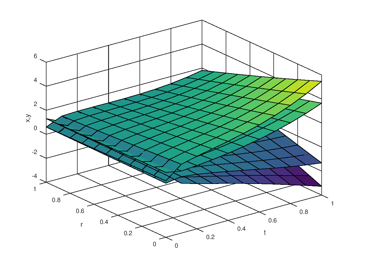
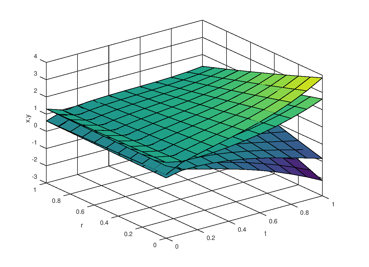
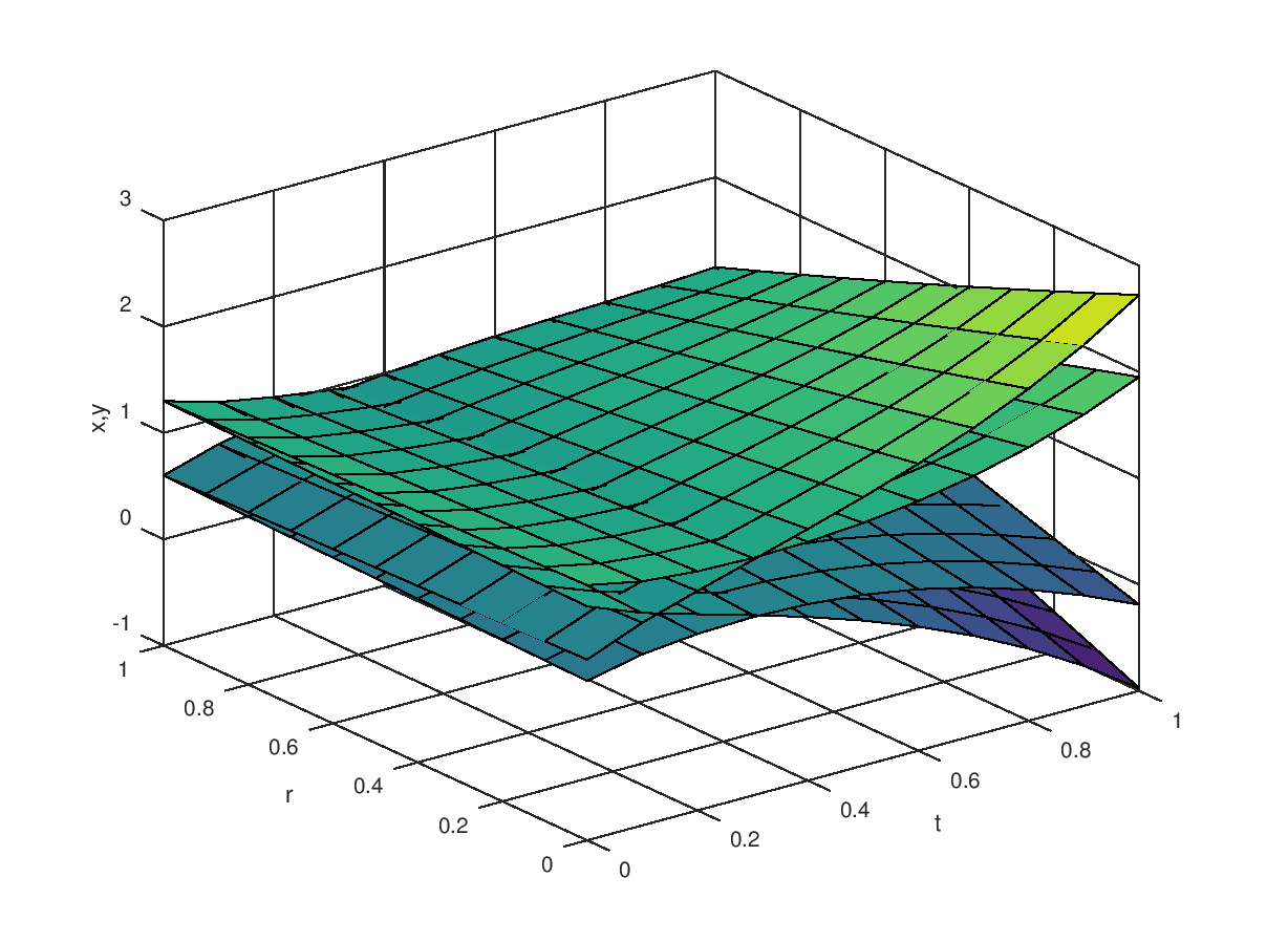
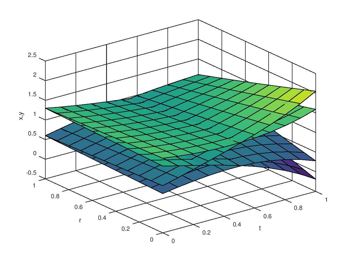
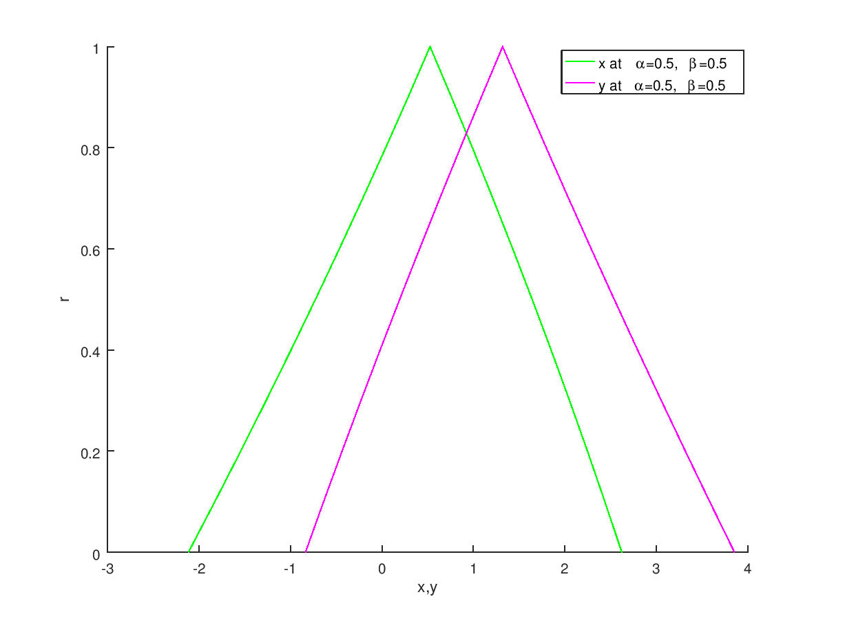
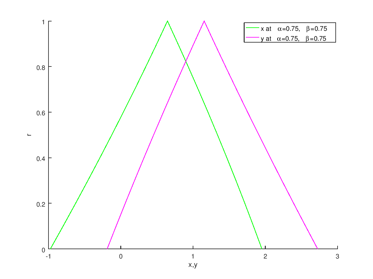
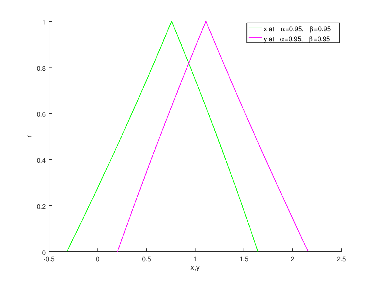
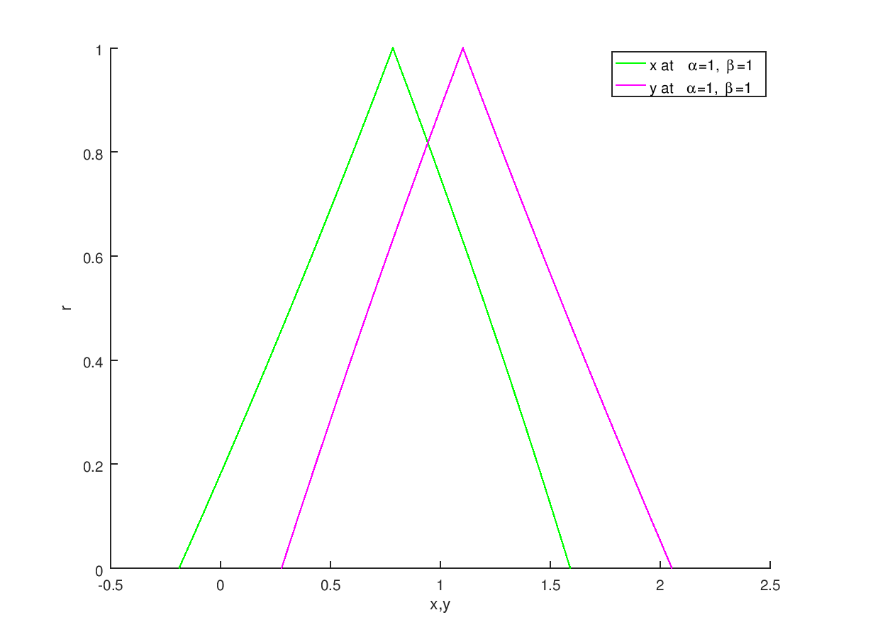
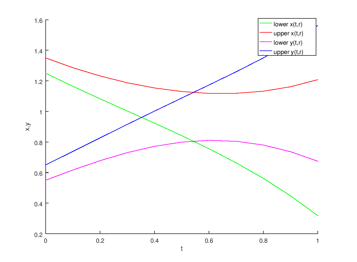
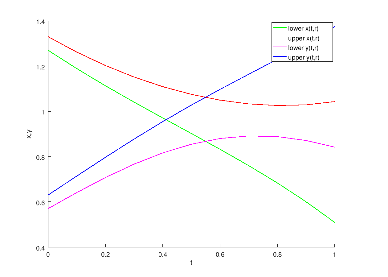
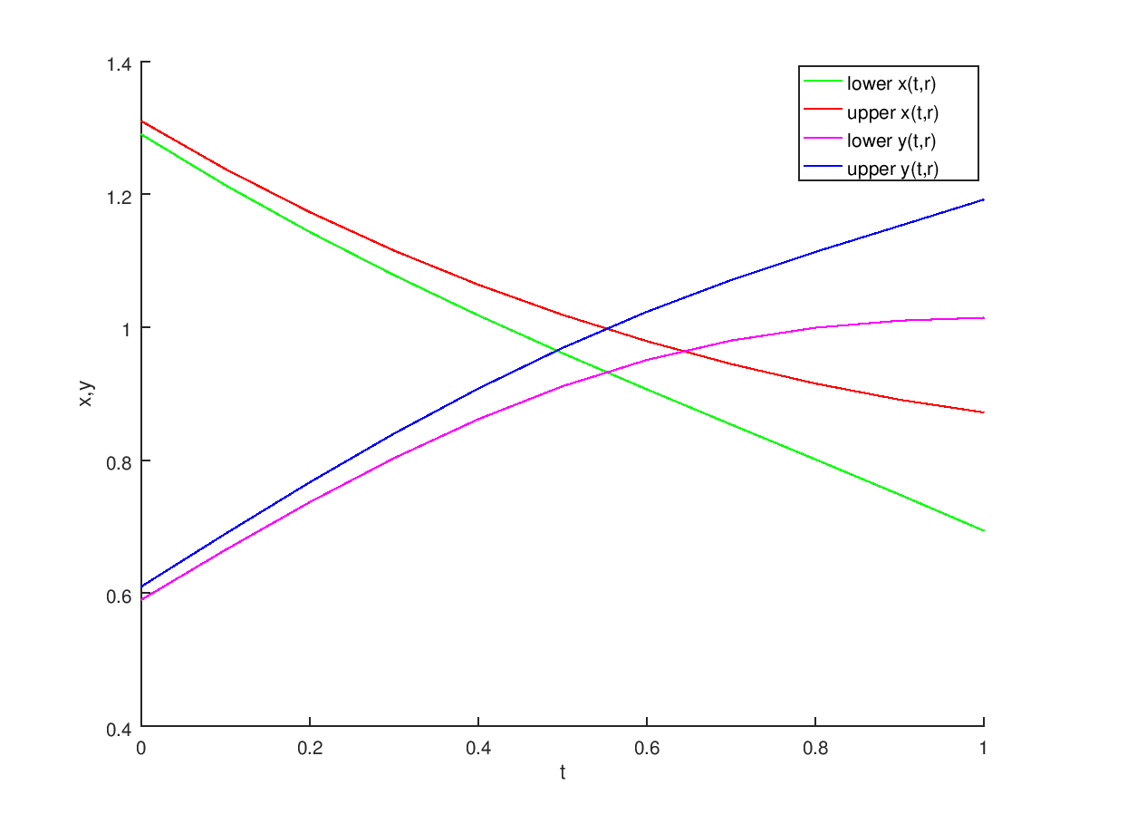
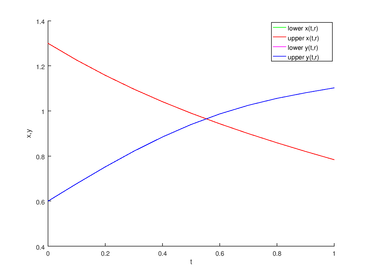
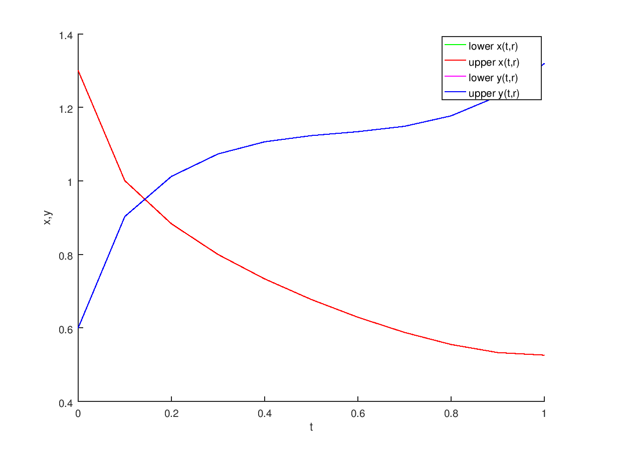
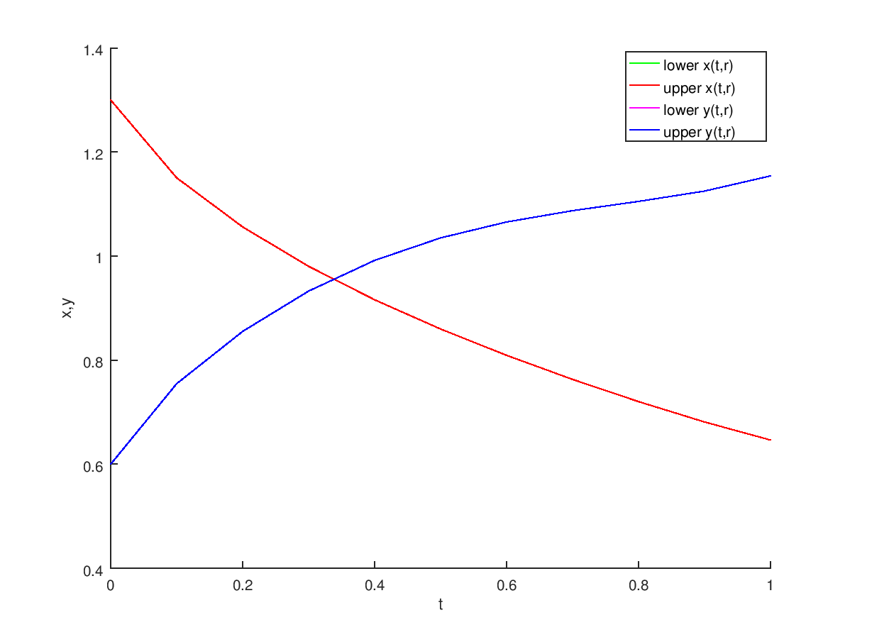
Numerical results are depicted in Figures 1- 12 respectively. In Figures 1- 4, by varying both $t$ and $r$ from 0 to 1 for $\alpha ,\beta =0.25,\alpha ,\beta =0.5,\alpha ,\beta =0.75,$ and $\alpha ,\beta =1.$ 3D results are depicted. In Figures 5-8, 2D figures are depicted by varying $r$ from 0 to 1 and t as constant $(t=1)$ for different values of fractional order. It can be concluded that the crisp solution lies in between the lower and upper bounds of the fuzzy solution. In Figures 9-12, 2D figures are depicted by varying $t$ from 0 to 1 for different values $r$ . The above figures noted that the lower and upper bounds of the fuzzy solutions are the same for $r=1$ .

The main focus of this work is to find the approximate solution for the system of fuzzy fractional differential equations. Predator-prey model is the most important application in the field of differential equations. The construction of the Shehu Adomian decomposition method is used to solve fuzzy fractional predator-prey equations. The proposed method is easy to implement and applicable for solving both linear and nonlinear fuzzy fractional differential equations. The given figures show the efficiency of the proposed method.

References

1Adomian, G. (1988). A review of the decomposition method in applied mathematics. Journal of Mathematical Analysis and Applications, 135, 501–544.
2Agarwal, R. P., Lakshmikantham, V., & Nieto, J. J. (2010). On the concept of solution for fractional differential equations with uncertainty. Nonlinear Analysis: Theory, Methods & Applications, 72, 2859–2862.
3Khalouta, A., & Kadem, A. (2019). A new method to solve fractional differential equations: Inverse fractional Shehu transform method. International Journal of Applications and Applied Mathematics, 14(2), 926–941.
4Arfan, M., Shah, K., Abdeljawad, T., & Hammouch, Z. (2020). An efficient tool for solving two-dimensional fuzzy fractional-ordered heat equation. Numerical Methods for Partial Differential Equations.
5Chakraverty, S. (2016). Fuzzy Arbitrary Order Systems. John Wiley & Sons.
6Diamond, P., & Kloeden, P. (1994). Metric Spaces of Fuzzy Sets: Theory and Applications. World Scientific, Singapore.
7Baleanu, D., Machado, J. A. T., & Luo, A. C. J. (2012). Fractional Dynamics and Control. Springer, New York.
8Goetschel, R. Jr., & Voxman, W. (1986). Elementary fuzzy calculus. Fuzzy Sets and Systems, 18(1), 31–43.
9Sharmila, R. G., & Savla, S. L. (2021). Shehu transform method for linear fuzzy fractional differential equations. Compliance Engineering Journal, 12(1).
10Sharmila, R. G., & Savla, S. L. (2023). Numerical solution for fuzzy fractional differential equations using fuzzy fractional fourth order Runge–Kutta method based on root mean square and contraharmonic mean. Ratio Mathematica, 49, 51–68.
11Podlubny, I. (1999). Fractional Differential Equations: An Introduction to Fractional Derivatives, Fractional Differential Equations, to Methods of Their Solution and Some of Their Applications. Academic Press, San Diego.
12Sumiati, I., Sukono, Kalfin, & Abdul, T. (2020). Solution of fractional ordinary differential equations using the Elzaki–Adomian decomposition method. In Proceedings of the 5th International Conference on Industrial and Operations Management (USA, August 10–14).
13Lydia, K. S. (2019). Solving system of nonlinear fractional differential equations using Mahgoub Adomian decomposition method. Bulletin of Pure and Applied Sciences, 38E(1), 396–404.
14Miller, K. S., & Ross, B. (1993). An Introduction to the Fractional Calculus and Fractional Differential Equations. John Wiley & Sons, New York.
15Savla, S. L., & Sharmila, R. G. (2023). Solving fuzzy fractional biological population model using Shehu Adomian decomposition method. Indian Journal of Science and Technology, 16(Special Issue 3), 44–54.
16Savla, S. L., Sharmila, R. G., & Kanna, T. (2026). Fuzzy fractional predator–prey model: A numerical approach using fuzzy fractional fourth-order Runge–Kutta method. Discontinuity, Nonlinearity, and Complexity, 15(4), 579–595.